Getting started with pymccrgb
This notebook shows an example of classifying a point cloud from a photogrammetric survey.
It uses the read_las and write_las functions for I/O and shows how to use mcc_rgb to classify points.
[1]:
import warnings
warnings.filterwarnings('ignore')
[2]:
import matplotlib.pyplot as plt
[3]:
from pymccrgb import mcc_rgb
from pymccrgb.plotting import plot_points_3d
from pymccrgb.ioutils import read_las, write_las
First, we load a dataset. In this case, it’s a point cloud produced from unmanned aerial vehicle (UAV) photography. The whole dataset is over 600K points, but let’s use the nrows argument to read a subset of the data.
[4]:
data = read_las('data/uav.las', nrows=2.5e5)
[5]:
print(data.shape)
(250000, 6)
We loaded 250K points with three color channels.
[6]:
plot_points_3d(data)
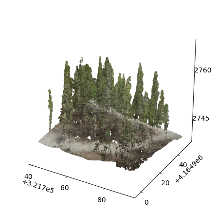
We can use the MCC-RGB algorithm (mcc-rgb) to classify the points by relative height and color.
In this example, let’s use a training height of 1 meter to capture canopy points. The algorithm will use points above 1 m relative height to train a non-ground classifier.
[7]:
ground, labels = mcc_rgb(data,
                         scales=[0.5, 1.0, 1.5],  # Scale domains (interpolation spacing)
                         tols=[1.0, 1.0, 1.0],    # Height tolerances
                         training_tols=[1.0],     # MCC-RGB training height
                         verbose=True)
--------------------
MCC step
--------------------
Scale: 0.50, Relative height: 1.0e+00, iter: 0
Removed 88342 nonground points (35.45 %)
--------------------
Classification update step
--------------------
Scale: 0.50, Relative height: 1.0e+00
Removed 47155 nonground points (18.92 %)
--------------------
MCC step
--------------------
Scale: 0.50, Relative height: 1.0e+00, iter: 1
Removed 5961 nonground points (2.39 %)
--------------------
MCC step
--------------------
Scale: 0.50, Relative height: 1.0e+00, iter: 2
Removed 1443 nonground points (0.58 %)
--------------------
MCC step
--------------------
Scale: 1.00, Relative height: 1.0e+00, iter: 0
Removed 1106 nonground points (0.44 %)
--------------------
MCC step
--------------------
Scale: 1.00, Relative height: 1.0e+00, iter: 1
Removed 298 nonground points (0.12 %)
--------------------
MCC step
--------------------
Scale: 1.00, Relative height: 1.0e+00, iter: 2
Removed 103 nonground points (0.04 %)
--------------------
MCC step
--------------------
Scale: 1.50, Relative height: 1.0e+00, iter: 0
Removed 535 nonground points (0.21 %)
--------------------
MCC step
--------------------
Scale: 1.50, Relative height: 1.0e+00, iter: 1
Removed 55 nonground points (0.02 %)
--------------------
MCC step
--------------------
Scale: 1.50, Relative height: 1.0e+00, iter: 2
Removed 1 nonground points (0.00 %)

Retained 104233 ground points (41.69 %)
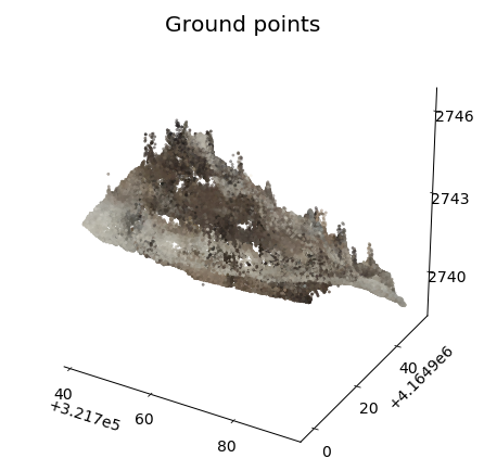
We can plot the ground and non-ground points with a plotting function.
[8]:
plot_points_3d(ground)
_ = plt.gca().set_title('Ground points')
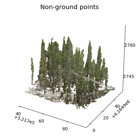
[9]:
plot_points_3d(data[labels == 0, :])
_ = plt.gca().set_title('Non-ground points')
[10]:
nground = (labels == 1).sum()
nnonground = (labels == 0).sum()
print(f"Classified {nground} ground points and {nnonground} non-ground points")
Classified 104233 ground points and 145767 non-ground poitns
Finally, you can save the output as a LAS file with write_las (or use numpy.save).
[11]:
write_las(ground, 'data/uav_ground.las')