MCC-RGB walkthrough

This notebook goes through the feature calculation and training steps of MCC-RGB to show the details behind the algorithm’s update step. It also shows how the parameters for the radial basis function (RBF) kernel transformation and stochastic gradient descent (SGD) classifier can be selected with cross-validation.

import warnings
warnings.filterwarnings('ignore')

import numpy as np

import matplotlib.pyplot as plt

from skimage.color import rgb2lab
from skimage.exposure import rescale_intensity

from sklearn.kernel_approximation import RBFSampler
from sklearn.linear_model import SGDClassifier
from sklearn.model_selection import GridSearchCV
from sklearn.pipeline import Pipeline

from pymccrgb.core import classify_ground_mcc
from pymccrgb.datasets import load_mammoth_lidar
from pymccrgb.plotting import plot_points_3d

Color features

First, the default color features are calculated for each point. These are a and b color values from CIE-Lab color space and a green-red normalized difference index (NGRDVI). In RGB or CIR data, these features highlight green canopy points.

data = load_mammoth_lidar(npoints=1e5)

rgb = rescale_intensity(data[:, 3:6], out_range="uint8").astype(np.uint8)
red = rgb[:, 0]
green = rgb[:, 1]
blue = rgb[:, 2]
ngrdvi = (green - red) / (green + red)
lab = rgb2lab(np.array([rgb]))[0]
X = np.hstack([lab[:, 1:3].reshape(-1, 2), ngrdvi.reshape(-1, 1)])

xx = data[:, 0]
yy = data[:, 1]
zz = data[:, 2]

1. MCC ground classification

The algorithm starts with a ground classification based on relative height as in a single MCC iteration. A spline surface is interpolated through the data with grid resolution scale. High points are classified as non-ground if they lie at least tol untis above this surface. The result is a vector of point labels y.

MCC iterates over interpolation scales and height tolerances, removing non-ground points until a stopping condition is reached.

For more details, see the MCC paper and mcc-lidar codebase.

scale = 1  # m
tol = 0.3  # m
labels = classify_ground_mcc(data, scale, tol)
y = labels

keep = np.isfinite(X).all(axis=-1)
X = X[keep, :]
y = y[keep]
data = data[keep, :]

2. MCC-RGB update step

The goal of MCC-RGB is to refine the current MCC classification using the non-ground class. To do this, the color features from the point cloud are used to train a binary classifier trained using MCC class labels.

Then, MCC ground points are re-classified using this classifier. If their predicted class is non-ground, they are re-labeled as non-ground points and removed before the next MCC iteration.

np.random.seed(10)
n_train = 1000
subset = np.random.choice(len(y), size=n_train)

X_train = X[subset, :]
y_train = y[subset]

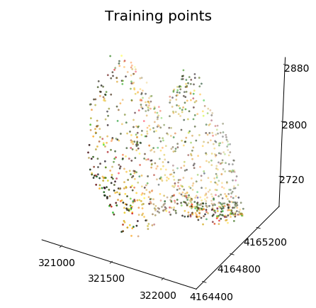
print(f"Training points - Ground: {np.sum(y_train)} Nonground: {np.sum(y_train == 0)}")

Training points - Ground: 663 Nonground: 337

plot_points_3d(data[subset, :])
plt.gca().set_title("Training points")

Text(0.5, 0.92, 'Training points')

Cross-validation can be used to determine reasonable values for the classifier parameters.

pipe = Pipeline([('rbf', RBFSampler()), ('clf', SGDClassifier(max_iter=10, n_jobs=-1))])

gammas = [0.01, 0.1, 1, 10, 100, 1000]
n_components = [10, 100, 1000]
Cs = [0.0001, 0.001, 0.01, 0.1, 1, 10, 100, 1000]
param_grid = {'rbf__n_components': n_components,
              'rbf__gamma': gammas,
              'clf__alpha': Cs
             }

grid = GridSearchCV(pipe, cv=5, n_jobs=-1, param_grid=param_grid)

grid.fit(X_train, y_train)

/home/rmsare/miniconda3/envs/pymcc/lib/python3.6/site-packages/sklearn/model_selection/_search.py:813: DeprecationWarning: The default of the `iid` parameter will change from True to False in version 0.22 and will be removed in 0.24. This will change numeric results when test-set sizes are unequal.
  DeprecationWarning)

GridSearchCV(cv=5, error_score='raise-deprecating',
             estimator=Pipeline(memory=None,
                                steps=[('rbf',
                                        RBFSampler(gamma=1.0, n_components=100,
                                                   random_state=None)),
                                       ('clf',
                                        SGDClassifier(alpha=0.0001,
                                                      average=False,
                                                      class_weight=None,
                                                      early_stopping=False,
                                                      epsilon=0.1, eta0=0.0,
                                                      fit_intercept=True,
                                                      l1_ratio=0.15,
                                                      learning_rate='optimal',
                                                      loss='hinge', max_iter=10,
                                                      n_iter_...
                                                      random_state=None,
                                                      shuffle=True, tol=0.001,
                                                      validation_fraction=0.1,
                                                      verbose=0,
                                                      warm_start=False))],
                                verbose=False),
             iid='warn', n_jobs=-1,
             param_grid={'clf__alpha': [0.0001, 0.001, 0.01, 0.1, 1, 10, 100,
                                        1000],
                         'rbf__gamma': [0.01, 0.1, 1, 10, 100, 1000],
                         'rbf__n_components': [10, 100, 1000]},
             pre_dispatch='2*n_jobs', refit=True, return_train_score=False,
             scoring=None, verbose=0)

print(grid.best_params_)

{'clf__alpha': 0.001, 'rbf__gamma': 0.01, 'rbf__n_components': 1000}

In this example, high-dimensional RBF features with 1000 components will be derived from the color features using an RFB transformation wit hgamma value 0.01. A stochastic gradient descent classifier is trained on these features using the MCC ground/non-ground labels.

pipe = Pipeline([('rbf', RBFSampler(n_components=1000, gamma=0.01)), ('clf', SGDClassifier(alpha=0.001, max_iter=10, n_jobs=-1))])

pipe.fit(X_train, y_train)

Pipeline(memory=None,
         steps=[('rbf',
                 RBFSampler(gamma=10, n_components=1000, random_state=None)),
                ('clf',
                 SGDClassifier(alpha=0.0001, average=False, class_weight=None,
                               early_stopping=False, epsilon=0.1, eta0=0.0,
                               fit_intercept=True, l1_ratio=0.15,
                               learning_rate='optimal', loss='hinge',
                               max_iter=10, n_iter_no_change=5, n_jobs=-1,
                               penalty='l2', power_t=0.5, random_state=None,
                               shuffle=True, tol=0.001, validation_fraction=0.1,
                               verbose=0, warm_start=False))],
         verbose=False)

Finally, MCC-RGB update steps use the predictions of the color-based classifier to update the original MCC ground points.

y_pred = pipe.predict(X)

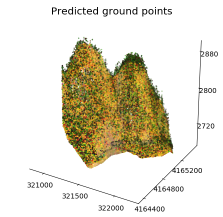
The color-based classifier produces another binary classification of the point cloud, shown below.

mask = y_pred == 1
plot_points_3d(data[mask, :])
plt.title('Predicted ground points')

Text(0.5, 0.92, 'Predicted ground points')

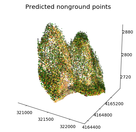
mask = y_pred == 0
plot_points_3d(data[mask, :])
plt.title('Predicted nonground points')

Text(0.5, 0.92, 'Predicted nonground points')

The color-based non-ground classification is used to update the original MCC ground points. If an MCC ground point is re-classified as non-ground by the MCC-RGB classifier, its class is updated to non-ground.

In practice, low vegetation, shadow, and low canopy points are usually updated - they share color similarity with higher vegetation points despite having low relative height.

mask = (y_pred == 0) & (y == 1)
plot_points_3d(data[mask, :])
plt.title('Updated MCC ground points')

Text(0.5, 0.92, 'Updated MCC ground points')

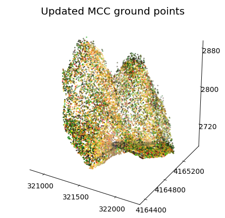
This is an example of a single iteration of the MCC-RGB classify-update procedure. The ground-only point cloud above is decimated further in later iterations.

The algorithm implemented in mcc_rgb continues to iterate over ground points until a stopping condition is reached (when only a small number of non-ground points are classified).